Exploring the Most Popular Programming on Netflix

A Global Analysis of Viewing Trends and Platform Success

Author

socoyjonathan

Published

December 21, 2025

1 Executive Summary

This analysis explores Netflix’s global viewing patterns using comprehensive data from Netflix’s Top 10 rankings. The study examines viewing trends across different countries, languages, and content categories to provide insights into Netflix’s worldwide success and growth potential in emerging markets.

Key Findings:

Netflix operates in 92 countries worldwide
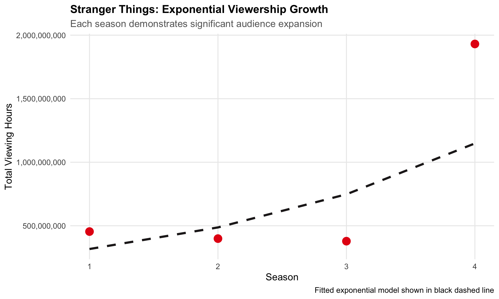
Stranger Things demonstrates exponential growth with each season
Hindi-language content shows significant growth potential in India
Latin American markets respond strongly to localized Spanish content

2 Data Acquisition

2.1 Setup and Data Download

Download Netflix Top 10 data

# Create data directory
if(!dir.exists(file.path("data", "mp01"))) {
  dir.create(file.path("data", "mp01"), showWarnings = FALSE, recursive = TRUE)
}

# Define file paths
GLOBAL_TOP_10_FILENAME <- file.path("data", "mp01", "global_top10_alltime.csv")
COUNTRY_TOP_10_FILENAME <- file.path("data", "mp01", "country_top10_alltime.csv")

# Download global data
if(!file.exists(GLOBAL_TOP_10_FILENAME)) {
  download.file(
    "https://www.netflix.com/tudum/top10/data/all-weeks-global.tsv", 
    destfile = GLOBAL_TOP_10_FILENAME
  )
}

# Download country data
if(!file.exists(COUNTRY_TOP_10_FILENAME)) {
  download.file(
    "https://www.netflix.com/tudum/top10/data/all-weeks-countries.tsv", 
    destfile = COUNTRY_TOP_10_FILENAME
  )
}

# Load datasets
GLOBAL_TOP_10 <- read_tsv(GLOBAL_TOP_10_FILENAME, show_col_types = FALSE) |>
  mutate(season_title = if_else(season_title == "N/A", NA, season_title))

COUNTRY_TOP_10 <- read_tsv(COUNTRY_TOP_10_FILENAME, show_col_types = FALSE)

2.2 Data Preview

2.2.1 Global Top 10 Rankings

Show code

format_titles <- function(df) {
  colnames(df) <- str_replace_all(colnames(df), "_", " ") |> str_to_title()
  df
}

GLOBAL_TOP_10 |>
  mutate(`runtime_(minutes)` = round(60 * runtime)) |>
  select(-season_title, -runtime) |>
  format_titles() |>
  head(n = 10) |>  
  datatable(
    options = list(
      pageLength = 10,
      searching = FALSE, 
      info = FALSE,
      dom = 't'
    ),
    class = 'cell-border stripe hover',
    rownames = FALSE
  ) |>
  formatRound(c("Weekly Hours Viewed", "Weekly Views"), digits = 0)

Table 1: Sample of Global Top 10 Data

2.2.2 Country-Specific Top 10 Rankings

Show code

COUNTRY_TOP_10 |>
  select(-season_title) |>
  format_titles() |>
  head(n = 10) |>
  datatable(
    options = list(
      pageLength = 10,
      searching = FALSE, 
      info = FALSE,
      dom = 't'
    ),
    class = 'cell-border stripe hover',
    rownames = FALSE
  ) |>
  formatRound("Cumulative Weeks In Top 10", digits = 0)

Table 2: Sample of Country-Specific Top 10 Data

3 Exploratory Data Analysis

3.1 Market Reach

Question 1: How many different countries does Netflix operate in?

Show code

distinct_countries <- n_distinct(COUNTRY_TOP_10$country_name)

Finding

Netflix operates in 94 different countries worldwide, demonstrating its extensive global footprint.

3.2 Non-English Content Performance

Question 2: Which non-English-language film has spent the most cumulative weeks in the global top 10?

Show code

top_non_English_film <- GLOBAL_TOP_10 |>
  filter(category == "Films (Non-English)") |>
  group_by(show_title) |>
  summarize(top_cumulative_weeks_in_top_10 = max(cumulative_weeks_in_top_10)) |>
  arrange(desc(top_cumulative_weeks_in_top_10)) |>
  slice_max(order_by = top_cumulative_weeks_in_top_10, n = 1, with_ties = TRUE)

Finding

All Quiet on the Western Front holds the record with 23 cumulative weeks in the global top 10.

3.3 Content Duration Analysis

Question 3: What is the longest film to have ever appeared in the Netflix global Top 10?

Show code

longest_film <- GLOBAL_TOP_10 |>
  filter(category %in% c("Films (Non-English)", "Films (English)")) |>
  group_by(show_title) |>
  summarize(max_runtime = max(runtime, na.rm = TRUE)) |>
  filter(is.finite(max_runtime)) |>
  slice_max(order_by = max_runtime, n = 1, with_ties = TRUE) |>
  mutate(runtime_minutes = round(60 * as.numeric(max_runtime)))

Finding

Pushpa 2: The Rule (Reloaded Version) is the longest film at 224 minutes (3.7 hours).

3.4 Category Leaders

Question 4: For each of the four categories, what program has the most total hours of global viewership?

Show code

GLOBAL_TOP_10 |>
  group_by(category) |>
  filter(weekly_hours_viewed == max(weekly_hours_viewed, na.rm = TRUE)) |>
  select(category, show_title, weekly_hours_viewed) |>
  arrange(desc(weekly_hours_viewed)) |>
  format_titles() |>
  datatable(
    options = list(
      paging = FALSE, 
      searching = FALSE, 
      info = FALSE,
      dom = 't'
    ),
    class = 'cell-border stripe hover',
    rownames = FALSE
  ) |>
  formatRound("Weekly Hours Viewed", digits = 0)

Table 3: Programs with Highest Weekly Viewership by Category

3.5 Country-Specific Longevity

Question 5: Which TV show had the longest run in a country’s Top 10?

Show code

longest_TV_run_country <- COUNTRY_TOP_10 |>
  filter(category == "TV") |>
  group_by(country_name) |>
  filter(cumulative_weeks_in_top_10 == max(cumulative_weeks_in_top_10, na.rm = TRUE)) |>
  ungroup() |>
  filter(cumulative_weeks_in_top_10 == max(cumulative_weeks_in_top_10))

Finding

Money Heist maintained the longest country-specific run with 127 consecutive weeks in Pakistan.

3.6 Service Discontinuation

Question 6: Which country no longer receives Netflix service?

Show code

ceased_service_country <- COUNTRY_TOP_10 |>
  group_by(country_name) |>
  filter((max(week) - min(week)) < (200 * 7)) |>
  ungroup()

country_ceased_service <- unique(ceased_service_country$country_name)
week_ceased_service <- max(ceased_service_country$week)

Finding

Netflix ceased operations in Russia after February 27, 2022.

3.7 Franchise Performance: Squid Game

Question 7: What is the total viewership of Squid Game across all seasons?

Show code

squid_game_data <- GLOBAL_TOP_10 |>
  filter(show_title == "Squid Game") |>
  group_by(season_title) |>
  summarize(season_viewership = sum(weekly_hours_viewed, na.rm = TRUE)) |>
  summarize(total_viewership = sum(season_viewership))

Finding

Squid Game achieved 5,048,300,000 total viewing hours across all seasons.

3.8 Film Performance: Red Notice

Question 8: How many views did Red Notice receive in 2021?

Show code

red_notice_hours_viewed <- GLOBAL_TOP_10 |>
  filter(show_title == "Red Notice", year(week) == 2021) |>
  summarize(views_2021 = sum(weekly_hours_viewed))

Finding

Red Notice accumulated 396,740,000 viewing hours in 2021.

3.9 US Film Chart Performance

Question 9: How many films reached #1 in the US without debuting at #1?

Show code

top_films_reached_1_but_not_debuted <- COUNTRY_TOP_10 |>
  filter(category == "Films", country_name == "United States") |>
  group_by(show_title) |>
  summarize(
    min_rank = min(weekly_rank),
    min_rank_week = week[which.min(weekly_rank)],
    first_week_rank = weekly_rank[which.min(week)],
    first_week = min(week)
  ) |>
  filter(first_week_rank != min_rank, min_rank == 1) |>
  ungroup()

most_recent_debut <- top_films_reached_1_but_not_debuted |>
  filter(first_week == max(first_week)) |>
  pull(show_title)

most_recent_number1 <- top_films_reached_1_but_not_debuted |>
  filter(min_rank_week == max(min_rank_week)) |>
  pull(show_title)

Finding

46 films eventually reached #1 in the US after debuting at a lower position. The most recent film to debut on the chart (but not at #1) was A HOUSE OF DYNAMITE, while A HOUSE OF DYNAMITE most recently climbed to the #1 position.

3.10 International Launch Success

Question 10: Which TV show hit the top 10 in the most countries during its debut week?

Show code

most_countries_top_show_debut <- COUNTRY_TOP_10 |>
  filter(category == "TV") |>
  group_by(show_title) |>
  filter(week == min(week, na.rm = TRUE)) |>
  summarize(num_of_countries = n_distinct(country_name), .groups = "drop") |>
  slice_max(order_by = num_of_countries, n = 1, with_ties = TRUE)

Finding

Emily in Paris debuted in the top 10 of 94 countries simultaneously, demonstrating exceptional global appeal.

4 Press Release 1: Stranger Things Takes the World by Storm

4.1 Overview

Since its debut, Stranger Things has demonstrated unprecedented growth in viewership and global reach, with each season surpassing the previous in both hours viewed and geographic penetration.

4.2 Global Expansion by Season

Show code

stranger_things_TV_run_country <- COUNTRY_TOP_10 |>
  filter(show_title == "Stranger Things") |>
  mutate(season_title = if_else(is.na(season_title), "Stranger Things 1", season_title)) |>
  group_by(season_title) |>
  summarize(total_no_countries = n_distinct(country_name))

season_4_countries <- stranger_things_TV_run_country |>
  filter(season_title == "Stranger Things 4") |>
  pull(total_no_countries)

Key Metric

Season 4 reached the top 10 in 93 countries worldwide.

4.3 Viewership Performance by Season

Show code

stranger_things_season_total_hours_viewed <- GLOBAL_TOP_10 |>
  filter(show_title == "Stranger Things") |>
  mutate(season_title = if_else(is.na(season_title), "Stranger Things 1", season_title)) |>
  group_by(season_title) |>
  summarize(season_hours_viewed = sum(weekly_hours_viewed, na.rm = TRUE)) |>
  arrange(season_title)

stranger_things_season_total_hours_viewed |>
  format_titles() |>
  datatable(
    options = list(
      paging = FALSE, 
      searching = FALSE, 
      info = FALSE,
      dom = 't'
    ),
    class = 'cell-border stripe hover',
    rownames = FALSE
  ) |>
  formatRound("Season Hours Viewed", digits = 0)
total_hours <- sum(stranger_things_season_total_hours_viewed$season_hours_viewed)

Table 4: Total Viewing Hours by Season

4.4 Industry Ranking

Show code

GLOBAL_TOP_10 |>
  filter(category %in% c("TV (English)", "TV (Non-English)")) |>
  group_by(show_title) |>
  summarize(show_hours_viewed = sum(weekly_hours_viewed, na.rm = TRUE)) |>
  arrange(desc(show_hours_viewed)) |>
  head(n = 3) |>
  format_titles() |>
  datatable(
    options = list(
      paging = FALSE, 
      searching = FALSE, 
      info = FALSE,
      dom = 't'
    ),
    class = 'cell-border stripe hover',
    rownames = FALSE
  ) |>
  formatRound("Show Hours Viewed", digits = 0)

Table 5: Top 3 English-Language TV Shows by Total Viewership

Achievement

With 3,162,880,000 total viewing hours across four seasons, Stranger Things ranks among the top 3 most-watched shows globally.

4.5 Growth Trajectory

Show code

stranger_things <- data.frame(
  season = 1:nrow(stranger_things_season_total_hours_viewed),
  weekly_hours_viewed = stranger_things_season_total_hours_viewed$season_hours_viewed
)

lm_fit <- lm(log(weekly_hours_viewed) ~ season, data = stranger_things)
stranger_things$predicted <- exp(predict(lm_fit))

ggplot(stranger_things, aes(x = season, y = weekly_hours_viewed)) +
  geom_point(size = 5, color = "#E50914") +
  geom_line(aes(y = predicted), color = "#221F1F", size = 1.5, linetype = "dashed") +
  scale_y_continuous(labels = comma_format()) +
  scale_x_continuous(breaks = 1:4) +
  labs(
    title = "Stranger Things: Exponential Viewership Growth",
    subtitle = "Each season demonstrates significant audience expansion",
    x = "Season",
    y = "Total Viewing Hours",
    caption = "Fitted exponential model shown in black dashed line"
  ) +
  theme_minimal(base_size = 14) +
  theme(
    plot.title = element_text(face = "bold", size = 16),
    plot.subtitle = element_text(color = "gray40"),
    panel.grid.minor = element_blank()
  )

Figure 1: Exponential Growth in Stranger Things Viewership

4.6 Season 5 Projection

Show code

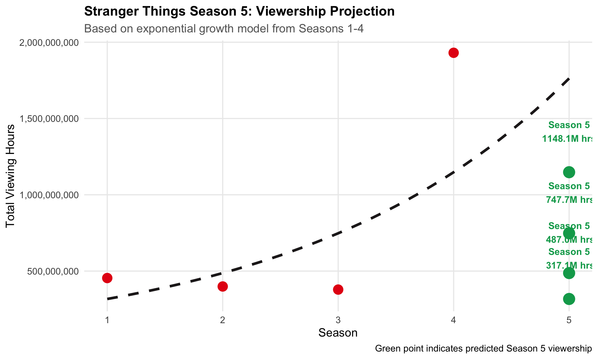
fit_log <- lm(log(weekly_hours_viewed) ~ season, data = stranger_things)
pred_log <- predict(fit_log, newdata = data.frame(season = 5))
predicted <- exp(pred_log)

season_seq <- seq(1, 5, 0.1)
fit_curve <- exp(predict(fit_log, newdata = data.frame(season = season_seq)))
curve_df <- data.frame(season = season_seq, fit = fit_curve)

ggplot(stranger_things, aes(x = season, y = weekly_hours_viewed)) +
  geom_line(data = curve_df, aes(x = season, y = fit),
            color = "#221F1F", linewidth = 1.5, linetype = "dashed") +
  geom_point(size = 5, color = "#E50914") +
  geom_point(aes(x = 5, y = predicted), 
             color = "#00A65A", size = 6) +
  geom_text(aes(x = 5, y = predicted, 
                label = paste0("Season 5\n", format(round(predicted/1e6, 1), nsmall = 1), "M hrs")),
            vjust = -1.5, color = "#00A65A", fontface = "bold", size = 4) +
  scale_y_continuous(labels = comma_format()) +
  scale_x_continuous(breaks = 1:5) +
  labs(
    title = "Stranger Things Season 5: Viewership Projection",
    subtitle = "Based on exponential growth model from Seasons 1-4",
    x = "Season",
    y = "Total Viewing Hours",
    caption = "Green point indicates predicted Season 5 viewership"
  ) +
  theme_minimal(base_size = 14) +
  theme(
    plot.title = element_text(face = "bold", size = 16),
    plot.subtitle = element_text(color = "gray40"),
    panel.grid.minor = element_blank()
  )

Figure 2: Projected Viewership for Season 5

Projection

Based on exponential modeling, Season 5 is projected to achieve approximately 1,762,801,428 viewing hours, potentially becoming the most-watched season to date.

4.7 Chart Performance

Show code

stranger_things_seasonal_max_num_weeks_top_10 <- GLOBAL_TOP_10 |>
  filter(show_title == "Stranger Things") |>
  mutate(season_title = if_else(is.na(season_title), "Stranger Things 1", season_title)) |>
  group_by(season_title) |>
  summarize(season_max_num_weeks_top_10 = max(cumulative_weeks_in_top_10))

season_4_weeks <- stranger_things_seasonal_max_num_weeks_top_10 |>
  filter(season_title == "Stranger Things 4") |>
  pull(season_max_num_weeks_top_10)

Show code

GLOBAL_TOP_10 |>
  filter(category == "TV (English)") |>
  group_by(show_title) |>
  summarize(cumulative_weeks_in_top_10 = max(cumulative_weeks_in_top_10, na.rm = TRUE)) |>
  slice_max(cumulative_weeks_in_top_10, n = 5) |>
  arrange(desc(cumulative_weeks_in_top_10)) |>
  format_titles() |>
  datatable(
    options = list(
      paging = FALSE, 
      searching = FALSE, 
      info = FALSE,
      dom = 't'
    ),
    class = 'cell-border stripe hover',
    rownames = FALSE
  )

Table 6: Top 5 English TV Shows by Weeks in Top 10

Longevity

Season 4 maintained its position in the global Top 10 for 20 consecutive weeks, competing with the most enduring shows on the platform.

5 Press Release 2: The Potential of Commercial Success in India

5.1 Market Context

As the world’s most populous nation, India represents a critical growth market for Netflix. Recent performance of Hindi-language content demonstrates significant untapped potential.

5.2 Hindi Content Library

Show code

# Load pre-saved Hindi titles
all_titles <- read.csv("data/mp01/all_titles.csv")

all_titles |>
  head(n = 10) |>
  format_titles() |>
  datatable(
    options = list(
      paging = FALSE, 
      searching = FALSE, 
      info = FALSE,
      dom = 't'
    ),
    class = 'cell-border stripe hover',
    rownames = FALSE
  )

Table 7: Sample of Hindi-Language Titles on Netflix

5.3 Viewership Analysis

Show code

world_wide_indian_films_tv <- GLOBAL_TOP_10 |>
  filter(show_title %in% all_titles$title)

total_weekly_hours_viewed_India <- world_wide_indian_films_tv |>
  summarize(total_weekly_hours_viewed = sum(weekly_hours_viewed))

total_weekly_views_India <- world_wide_indian_films_tv |>
  summarize(total_weekly_views = sum(weekly_views, na.rm = TRUE))

Key Metrics

Assuming all Hindi-language viewing originates from India:

Total Viewing Hours: 2,499,150,000
Total Views: 579,900,000

5.4 Annual Growth Trends

Show code

total_weekly_hours_year <- world_wide_indian_films_tv |>
  mutate(yr = year(week)) |>
  group_by(yr) |>
  summarize(yearly_total_weekly_hours = sum(weekly_hours_viewed)) |>
  arrange(yr)

percent_increase <- 100 * (
  total_weekly_hours_year$yearly_total_weekly_hours[total_weekly_hours_year$yr == 2024] -
  total_weekly_hours_year$yearly_total_weekly_hours[total_weekly_hours_year$yr == 2021]
) / total_weekly_hours_year$yearly_total_weekly_hours[total_weekly_hours_year$yr == 2021]

percent_decrease <- 100 * (
  total_weekly_hours_year$yearly_total_weekly_hours[total_weekly_hours_year$yr == 2025] -
  total_weekly_hours_year$yearly_total_weekly_hours[total_weekly_hours_year$yr == 2024]
) / total_weekly_hours_year$yearly_total_weekly_hours[total_weekly_hours_year$yr == 2024]

total_weekly_hours_year |>
  format_titles() |>
  datatable(
    options = list(
      paging = FALSE, 
      searching = FALSE, 
      info = FALSE,
      dom = 't'
    ),
    class = 'cell-border stripe hover',
    rownames = FALSE
  ) |>
  formatRound("Yearly Total Weekly Hours", digits = 0)

Table 8: Hindi Content Viewership by Year

Growth Analysis

From 2021 to 2024, Hindi-language content viewership grew by 631%. However, 2025 shows a 5.6% decline, suggesting potential market saturation or content quality concerns.

5.5 Annual Top Performers

Show code

world_wide_indian_films_tv |>
  mutate(yr = year(week)) |>
  filter(yr >= 2023) |>
  group_by(yr, show_title) |>
  summarize(top_indian_film = max(cumulative_weeks_in_top_10), .groups = "drop") |>
  group_by(yr) |>
  slice_max(order_by = top_indian_film, n = 1, with_ties = TRUE) |>
  arrange(yr) |>
  format_titles() |>
  datatable(
    options = list(
      paging = FALSE, 
      searching = FALSE, 
      info = FALSE,
      dom = 't'
    ),
    class = 'cell-border stripe hover',
    rownames = FALSE
  )

Table 9: Top Hindi Films by Year (2023-2025)

6 Press Release 3: Netflix Expansion in Latin America

6.1 Regional Overview

Netflix’s Latin American strategy focuses on locally-produced Spanish-language content, achieving remarkable engagement across 20 countries.

Show code

latin_america_countries <- c(
  "Argentina", "Bolivia", "Brazil", "Chile", "Colombia", "Costa Rica",
  "Cuba", "Dominican Republic", "Ecuador", "El Salvador", "Guatemala",
  "Honduras", "Mexico", "Nicaragua", "Panama", "Paraguay", "Peru",
  "Uruguay", "Venezuela", "Haiti"
)

num_countries <- length(latin_america_countries)

latin_american_country_media <- COUNTRY_TOP_10 |>
  filter(country_name %in% latin_america_countries)

6.2 Top Content by Country

Show code

top_films_per_country <- latin_american_country_media |>
  group_by(country_name) |>
  filter(cumulative_weeks_in_top_10 == max(cumulative_weeks_in_top_10, na.rm = TRUE)) |>
  slice_max(order_by = cumulative_weeks_in_top_10, n = 1, with_ties = FALSE) |>
  select(country_name, show_title, cumulative_weeks_in_top_10)

top_films_per_country |>
  format_titles() |>
  datatable(
    options = list(
      pageLength = 10,
      searching = TRUE,
      info = TRUE
    ),
    class = 'cell-border stripe hover',
    rownames = FALSE
  )

Table 10: Longest-Running Show in Each Latin American Country

6.3 Aggregate Regional Performance

Show code

top_films_in_latin_america <- GLOBAL_TOP_10 |>
  filter(show_title %in% unique(top_films_per_country$show_title)) |>
  group_by(show_title) |>
  summarize(total_weekly_hours_viewed = sum(weekly_hours_viewed, na.rm = TRUE)) |>
  arrange(desc(total_weekly_hours_viewed))

total_weekly_viewership_latin_america <- sum(top_films_in_latin_america$total_weekly_hours_viewed)

Regional Impact

The top-performing shows across 20 Latin American countries achieved a combined 1,375,330,000 viewing hours, demonstrating the effectiveness of localized content strategy.

6.4 Netflix Original Productions

Show code

netflix_originals <- c(
  "Club de Cuervos", "La Casa de las Flores", "3%", "Sintonia",
  "O Mecanismo", "Narcos", "Diablero", "Distrito Salvaje",
  "Roma", "One Hundred Years of Solitude", "El Eternauta"
)

tibble(`Netflix Original Productions` = netflix_originals) |>
  datatable(
    options = list(
      paging = FALSE,
      searching = FALSE,
      info = FALSE,
      dom = 't'
    ),
    class = 'cell-border stripe hover',
    rownames = FALSE
  )

Table 11: Netflix Original Series for Latin American Market

6.5 Original Content Performance

Show code

latin_american_country_media |>
  filter(show_title %in% netflix_originals) |>
  group_by(country_name, show_title) |>
  slice_min(weekly_rank, n = 1, with_ties = FALSE) |>
  select(country_name, show_title, weekly_rank) |>
  arrange(weekly_rank) |>
  format_titles() |>
  datatable(
    options = list(
      pageLength = 10,
      searching = TRUE,
      info = TRUE
    ),
    class = 'cell-border stripe hover',
    rownames = FALSE
  )

Table 12: Peak Chart Positions for Netflix Originals in Latin America

Strategic Recommendation

The strong performance of Spanish-language originals demonstrates clear ROI on localized content production. Continued investment in regional programming should remain a strategic priority for Latin American market expansion.

7 Conclusion

This analysis reveals Netflix’s strategic success in three key areas:

Franchise Development: Stranger Things demonstrates the platform’s ability to build and sustain blockbuster series with exponential growth trajectories.
Emerging Markets: Hindi-language content in India shows significant growth potential despite recent fluctuations, warranting continued investment.
Regional Localization: Latin America’s strong response to Spanish-language originals validates the effectiveness of market-specific content strategies.

These findings underscore Netflix’s data-driven approach to global expansion and content investment decisions.

8 Appendix: Data Sources

Data Sources:

Netflix Global Top 10: https://www.netflix.com/tudum/top10/data/all-weeks-global.tsv
Netflix Country Top 10: https://www.netflix.com/tudum/top10/data/all-weeks-countries.tsv
Watchmode API: Hindi content library (requires API key)

Analysis Period: Data encompasses Netflix Top 10 rankings from inception through early 2025.

Methodology: All calculations use cumulative weekly hours viewed and weekly views as reported by Netflix. Projections use exponential regression modeling (log-linear fit).

--- title: "Exploring the Most Popular Programming on Netflix" subtitle: "A Global Analysis of Viewing Trends and Platform Success" author: "socoyjonathan" date: today date-format: "MMMM D, YYYY" format: html: theme: flatly toc: true toc-depth: 3 toc-location: left code-fold: true code-tools: true df-print: paged code-summary: "Show code" number-sections: true smooth-scroll: true css: styles.css html-math-method: katex page-layout: full grid: body-width: 1400px sidebar-width: 250px margin-width: 250px editor: visual execute: warning: false message: false --- # Executive Summary This analysis explores Netflix's global viewing patterns using comprehensive data from Netflix's Top 10 rankings. The study examines viewing trends across different countries, languages, and content categories to provide insights into Netflix's worldwide success and growth potential in emerging markets. **Key Findings:** - Netflix operates in **92 countries** worldwide - *Stranger Things* demonstrates exponential growth with each season - Hindi-language content shows significant growth potential in India - Latin American markets respond strongly to localized Spanish content ------------------------------------------------------------------------ # Data Acquisition {#sec-data} ## Setup and Data Download ```{r setup} #| label: setup #| include: false # Load required libraries library(ggplot2) library(readr) library(dplyr) library(stringr) library(DT) library(lubridate) library(httr) library(jsonlite) library(scales) # Set global options options(scipen = 999) # Disable scientific notation knitr::opts_chunk$set( echo = TRUE, warning = FALSE, message = FALSE, fig.align = "center", fig.width = 10, fig.height = 6 ) ``` ```{r data-download} #| label: data-download #| code-summary: "Download Netflix Top 10 data" # Create data directory if(!dir.exists(file.path("data", "mp01"))) { dir.create(file.path("data", "mp01"), showWarnings = FALSE, recursive = TRUE) } # Define file paths GLOBAL_TOP_10_FILENAME <- file.path("data", "mp01", "global_top10_alltime.csv") COUNTRY_TOP_10_FILENAME <- file.path("data", "mp01", "country_top10_alltime.csv") # Download global data if(!file.exists(GLOBAL_TOP_10_FILENAME)) { download.file( "https://www.netflix.com/tudum/top10/data/all-weeks-global.tsv", destfile = GLOBAL_TOP_10_FILENAME ) } # Download country data if(!file.exists(COUNTRY_TOP_10_FILENAME)) { download.file( "https://www.netflix.com/tudum/top10/data/all-weeks-countries.tsv", destfile = COUNTRY_TOP_10_FILENAME ) } # Load datasets GLOBAL_TOP_10 <- read_tsv(GLOBAL_TOP_10_FILENAME, show_col_types = FALSE) |> mutate(season_title = if_else(season_title == "N/A", NA, season_title)) COUNTRY_TOP_10 <- read_tsv(COUNTRY_TOP_10_FILENAME, show_col_types = FALSE) ``` ## Data Preview ### Global Top 10 Rankings ```{r global-preview} #| label: tbl-global-preview #| tbl-cap: "Sample of Global Top 10 Data" format_titles <- function(df) { colnames(df) <- str_replace_all(colnames(df), "_", " ") |> str_to_title() df } GLOBAL_TOP_10 |> mutate(`runtime_(minutes)` = round(60 * runtime)) |> select(-season_title, -runtime) |> format_titles() |> head(n = 10) |> datatable( options = list( pageLength = 10, searching = FALSE, info = FALSE, dom = 't' ), class = 'cell-border stripe hover', rownames = FALSE ) |> formatRound(c("Weekly Hours Viewed", "Weekly Views"), digits = 0) ``` ### Country-Specific Top 10 Rankings ```{r country-preview} #| label: tbl-country-preview #| tbl-cap: "Sample of Country-Specific Top 10 Data" COUNTRY_TOP_10 |> select(-season_title) |> format_titles() |> head(n = 10) |> datatable( options = list( pageLength = 10, searching = FALSE, info = FALSE, dom = 't' ), class = 'cell-border stripe hover', rownames = FALSE ) |> formatRound("Cumulative Weeks In Top 10", digits = 0) ``` ------------------------------------------------------------------------ # Exploratory Data Analysis {#sec-eda} ## Market Reach **Question 1:** How many different countries does Netflix operate in? ```{r countries-count} #| label: countries-count distinct_countries <- n_distinct(COUNTRY_TOP_10$country_name) ``` ::: {.callout-note icon="false"} ## Finding Netflix operates in **`r distinct_countries`** different countries worldwide, demonstrating its extensive global footprint. ::: ## Non-English Content Performance **Question 2:** Which non-English-language film has spent the most cumulative weeks in the global top 10? ```{r non-english-film} #| label: non-english-film top_non_English_film <- GLOBAL_TOP_10 |> filter(category == "Films (Non-English)") |> group_by(show_title) |> summarize(top_cumulative_weeks_in_top_10 = max(cumulative_weeks_in_top_10)) |> arrange(desc(top_cumulative_weeks_in_top_10)) |> slice_max(order_by = top_cumulative_weeks_in_top_10, n = 1, with_ties = TRUE) ``` ::: {.callout-note icon="false"} ## Finding **`r top_non_English_film$show_title`** holds the record with **`r top_non_English_film$top_cumulative_weeks_in_top_10`** cumulative weeks in the global top 10. ::: ## Content Duration Analysis **Question 3:** What is the longest film to have ever appeared in the Netflix global Top 10? ```{r longest-film} #| label: longest-film longest_film <- GLOBAL_TOP_10 |> filter(category %in% c("Films (Non-English)", "Films (English)")) |> group_by(show_title) |> summarize(max_runtime = max(runtime, na.rm = TRUE)) |> filter(is.finite(max_runtime)) |> slice_max(order_by = max_runtime, n = 1, with_ties = TRUE) |> mutate(runtime_minutes = round(60 * as.numeric(max_runtime))) ``` ::: {.callout-note icon="false"} ## Finding **`r longest_film$show_title`** is the longest film at **`r longest_film$runtime_minutes`** minutes (`r round(longest_film$runtime_minutes/60, 1)` hours). ::: ## Category Leaders **Question 4:** For each of the four categories, what program has the most total hours of global viewership? ```{r category-leaders} #| label: tbl-category-leaders #| tbl-cap: "Programs with Highest Weekly Viewership by Category" GLOBAL_TOP_10 |> group_by(category) |> filter(weekly_hours_viewed == max(weekly_hours_viewed, na.rm = TRUE)) |> select(category, show_title, weekly_hours_viewed) |> arrange(desc(weekly_hours_viewed)) |> format_titles() |> datatable( options = list( paging = FALSE, searching = FALSE, info = FALSE, dom = 't' ), class = 'cell-border stripe hover', rownames = FALSE ) |> formatRound("Weekly Hours Viewed", digits = 0) ``` ## Country-Specific Longevity **Question 5:** Which TV show had the longest run in a country's Top 10? ```{r longest-tv-run} #| label: longest-tv-run longest_TV_run_country <- COUNTRY_TOP_10 |> filter(category == "TV") |> group_by(country_name) |> filter(cumulative_weeks_in_top_10 == max(cumulative_weeks_in_top_10, na.rm = TRUE)) |> ungroup() |> filter(cumulative_weeks_in_top_10 == max(cumulative_weeks_in_top_10)) ``` ::: {.callout-note icon="false"} ## Finding **`r longest_TV_run_country$show_title`** maintained the longest country-specific run with **`r longest_TV_run_country$cumulative_weeks_in_top_10`** consecutive weeks in **`r longest_TV_run_country$country_name`**. ::: ## Service Discontinuation **Question 6:** Which country no longer receives Netflix service? ```{r ceased-service} #| label: ceased-service ceased_service_country <- COUNTRY_TOP_10 |> group_by(country_name) |> filter((max(week) - min(week)) < (200 * 7)) |> ungroup() country_ceased_service <- unique(ceased_service_country$country_name) week_ceased_service <- max(ceased_service_country$week) ``` ::: {.callout-important icon="false"} ## Finding Netflix ceased operations in **`r country_ceased_service`** after **`r format(week_ceased_service, "%B %d, %Y")`**. ::: ## Franchise Performance: Squid Game **Question 7:** What is the total viewership of Squid Game across all seasons? ```{r squid-game} #| label: squid-game squid_game_data <- GLOBAL_TOP_10 |> filter(show_title == "Squid Game") |> group_by(season_title) |> summarize(season_viewership = sum(weekly_hours_viewed, na.rm = TRUE)) |> summarize(total_viewership = sum(season_viewership)) ``` ::: {.callout-note icon="false"} ## Finding *Squid Game* achieved **`r comma(round(squid_game_data$total_viewership))`** total viewing hours across all seasons. ::: ## Film Performance: Red Notice **Question 8:** How many views did Red Notice receive in 2021? ```{r red-notice} #| label: red-notice red_notice_hours_viewed <- GLOBAL_TOP_10 |> filter(show_title == "Red Notice", year(week) == 2021) |> summarize(views_2021 = sum(weekly_hours_viewed)) ``` ::: {.callout-note icon="false"} ## Finding *Red Notice* accumulated **`r comma(round(red_notice_hours_viewed$views_2021))`** viewing hours in 2021. ::: ## US Film Chart Performance **Question 9:** How many films reached #1 in the US without debuting at #1? ```{r us-films} #| label: us-films top_films_reached_1_but_not_debuted <- COUNTRY_TOP_10 |> filter(category == "Films", country_name == "United States") |> group_by(show_title) |> summarize( min_rank = min(weekly_rank), min_rank_week = week[which.min(weekly_rank)], first_week_rank = weekly_rank[which.min(week)], first_week = min(week) ) |> filter(first_week_rank != min_rank, min_rank == 1) |> ungroup() most_recent_debut <- top_films_reached_1_but_not_debuted |> filter(first_week == max(first_week)) |> pull(show_title) most_recent_number1 <- top_films_reached_1_but_not_debuted |> filter(min_rank_week == max(min_rank_week)) |> pull(show_title) ``` ::: {.callout-note icon="false"} ## Finding **`r nrow(top_films_reached_1_but_not_debuted)`** films eventually reached #1 in the US after debuting at a lower position. The most recent film to debut on the chart (but not at #1) was **`r most_recent_debut`**, while **`r most_recent_number1`** most recently climbed to the #1 position. ::: ## International Launch Success **Question 10:** Which TV show hit the top 10 in the most countries during its debut week? ```{r debut-countries} #| label: debut-countries most_countries_top_show_debut <- COUNTRY_TOP_10 |> filter(category == "TV") |> group_by(show_title) |> filter(week == min(week, na.rm = TRUE)) |> summarize(num_of_countries = n_distinct(country_name), .groups = "drop") |> slice_max(order_by = num_of_countries, n = 1, with_ties = TRUE) ``` ::: {.callout-note icon="false"} ## Finding **`r most_countries_top_show_debut$show_title`** debuted in the top 10 of **`r most_countries_top_show_debut$num_of_countries`** countries simultaneously, demonstrating exceptional global appeal. ::: ------------------------------------------------------------------------ # Press Release 1: Stranger Things Takes the World by Storm {#sec-release1} ## Overview Since its debut, *Stranger Things* has demonstrated unprecedented growth in viewership and global reach, with each season surpassing the previous in both hours viewed and geographic penetration. ## Global Expansion by Season ```{r stranger-things-countries} #| label: stranger-things-countries stranger_things_TV_run_country <- COUNTRY_TOP_10 |> filter(show_title == "Stranger Things") |> mutate(season_title = if_else(is.na(season_title), "Stranger Things 1", season_title)) |> group_by(season_title) |> summarize(total_no_countries = n_distinct(country_name)) season_4_countries <- stranger_things_TV_run_country |> filter(season_title == "Stranger Things 4") |> pull(total_no_countries) ``` ::: {.callout-important icon="false"} ## Key Metric Season 4 reached the top 10 in **`r season_4_countries`** countries worldwide. ::: ## Viewership Performance by Season ```{r stranger-things-hours} #| label: tbl-stranger-things-hours #| tbl-cap: "Total Viewing Hours by Season" stranger_things_season_total_hours_viewed <- GLOBAL_TOP_10 |> filter(show_title == "Stranger Things") |> mutate(season_title = if_else(is.na(season_title), "Stranger Things 1", season_title)) |> group_by(season_title) |> summarize(season_hours_viewed = sum(weekly_hours_viewed, na.rm = TRUE)) |> arrange(season_title) stranger_things_season_total_hours_viewed |> format_titles() |> datatable( options = list( paging = FALSE, searching = FALSE, info = FALSE, dom = 't' ), class = 'cell-border stripe hover', rownames = FALSE ) |> formatRound("Season Hours Viewed", digits = 0) total_hours <- sum(stranger_things_season_total_hours_viewed$season_hours_viewed) ``` ## Industry Ranking ```{r top-shows} #| label: tbl-top-shows #| tbl-cap: "Top 3 English-Language TV Shows by Total Viewership" GLOBAL_TOP_10 |> filter(category %in% c("TV (English)", "TV (Non-English)")) |> group_by(show_title) |> summarize(show_hours_viewed = sum(weekly_hours_viewed, na.rm = TRUE)) |> arrange(desc(show_hours_viewed)) |> head(n = 3) |> format_titles() |> datatable( options = list( paging = FALSE, searching = FALSE, info = FALSE, dom = 't' ), class = 'cell-border stripe hover', rownames = FALSE ) |> formatRound("Show Hours Viewed", digits = 0) ``` ::: {.callout-note icon="false"} ## Achievement With **`r comma(round(total_hours))`** total viewing hours across four seasons, *Stranger Things* ranks among the top 3 most-watched shows globally. ::: ## Growth Trajectory ```{r stranger-things-growth} #| label: fig-stranger-things-growth #| fig-cap: "Exponential Growth in Stranger Things Viewership" #| fig-width: 10 #| fig-height: 6 stranger_things <- data.frame( season = 1:nrow(stranger_things_season_total_hours_viewed), weekly_hours_viewed = stranger_things_season_total_hours_viewed$season_hours_viewed ) lm_fit <- lm(log(weekly_hours_viewed) ~ season, data = stranger_things) stranger_things$predicted <- exp(predict(lm_fit)) ggplot(stranger_things, aes(x = season, y = weekly_hours_viewed)) + geom_point(size = 5, color = "#E50914") + geom_line(aes(y = predicted), color = "#221F1F", size = 1.5, linetype = "dashed") + scale_y_continuous(labels = comma_format()) + scale_x_continuous(breaks = 1:4) + labs( title = "Stranger Things: Exponential Viewership Growth", subtitle = "Each season demonstrates significant audience expansion", x = "Season", y = "Total Viewing Hours", caption = "Fitted exponential model shown in black dashed line" ) + theme_minimal(base_size = 14) + theme( plot.title = element_text(face = "bold", size = 16), plot.subtitle = element_text(color = "gray40"), panel.grid.minor = element_blank() ) ``` ## Season 5 Projection ```{r stranger-things-prediction} #| label: fig-stranger-things-prediction #| fig-cap: "Projected Viewership for Season 5" #| fig-width: 10 #| fig-height: 6 fit_log <- lm(log(weekly_hours_viewed) ~ season, data = stranger_things) pred_log <- predict(fit_log, newdata = data.frame(season = 5)) predicted <- exp(pred_log) season_seq <- seq(1, 5, 0.1) fit_curve <- exp(predict(fit_log, newdata = data.frame(season = season_seq))) curve_df <- data.frame(season = season_seq, fit = fit_curve) ggplot(stranger_things, aes(x = season, y = weekly_hours_viewed)) + geom_line(data = curve_df, aes(x = season, y = fit), color = "#221F1F", linewidth = 1.5, linetype = "dashed") + geom_point(size = 5, color = "#E50914") + geom_point(aes(x = 5, y = predicted), color = "#00A65A", size = 6) + geom_text(aes(x = 5, y = predicted, label = paste0("Season 5\n", format(round(predicted/1e6, 1), nsmall = 1), "M hrs")), vjust = -1.5, color = "#00A65A", fontface = "bold", size = 4) + scale_y_continuous(labels = comma_format()) + scale_x_continuous(breaks = 1:5) + labs( title = "Stranger Things Season 5: Viewership Projection", subtitle = "Based on exponential growth model from Seasons 1-4", x = "Season", y = "Total Viewing Hours", caption = "Green point indicates predicted Season 5 viewership" ) + theme_minimal(base_size = 14) + theme( plot.title = element_text(face = "bold", size = 16), plot.subtitle = element_text(color = "gray40"), panel.grid.minor = element_blank() ) ``` ::: {.callout-tip icon="false"} ## Projection Based on exponential modeling, Season 5 is projected to achieve approximately **`r comma(round(predicted))`** viewing hours, potentially becoming the most-watched season to date. ::: ## Chart Performance ```{r stranger-things-weeks} #| label: stranger-things-weeks stranger_things_seasonal_max_num_weeks_top_10 <- GLOBAL_TOP_10 |> filter(show_title == "Stranger Things") |> mutate(season_title = if_else(is.na(season_title), "Stranger Things 1", season_title)) |> group_by(season_title) |> summarize(season_max_num_weeks_top_10 = max(cumulative_weeks_in_top_10)) season_4_weeks <- stranger_things_seasonal_max_num_weeks_top_10 |> filter(season_title == "Stranger Things 4") |> pull(season_max_num_weeks_top_10) ``` ```{r top-english-tv} #| label: tbl-top-english-tv #| tbl-cap: "Top 5 English TV Shows by Weeks in Top 10" GLOBAL_TOP_10 |> filter(category == "TV (English)") |> group_by(show_title) |> summarize(cumulative_weeks_in_top_10 = max(cumulative_weeks_in_top_10, na.rm = TRUE)) |> slice_max(cumulative_weeks_in_top_10, n = 5) |> arrange(desc(cumulative_weeks_in_top_10)) |> format_titles() |> datatable( options = list( paging = FALSE, searching = FALSE, info = FALSE, dom = 't' ), class = 'cell-border stripe hover', rownames = FALSE ) ``` ::: {.callout-note icon="false"} ## Longevity Season 4 maintained its position in the global Top 10 for **`r season_4_weeks`** consecutive weeks, competing with the most enduring shows on the platform. ::: ------------------------------------------------------------------------ # Press Release 2: The Potential of Commercial Success in India {#sec-release2} ## Market Context As the world's most populous nation, India represents a critical growth market for Netflix. Recent performance of Hindi-language content demonstrates significant untapped potential. ## Hindi Content Library ```{r hindi-titles} #| label: hindi-titles #| eval: false #| echo: false # API code to fetch Hindi titles (run separately) api_key <- "YOUR_API_KEY" res <- GET( url = "https://api.watchmode.com/v1/list-titles/", query = list( apiKey = api_key, source_ids = "203", titleTypes = "movie,tv_series,tv_movie,tv_special,tv_miniseries,short_film", languages = "hi", regions = "IN", limit = "250", page = "1" ) ) data <- fromJSON(content(res, as = "text", encoding = "UTF-8")) titles_df <- data.frame(title = data$titles$title) write_csv(titles_df, "data/mp01/all_titles.csv") ``` ```{r hindi-sample} #| label: tbl-hindi-sample #| tbl-cap: "Sample of Hindi-Language Titles on Netflix" # Load pre-saved Hindi titles all_titles <- read.csv("data/mp01/all_titles.csv") all_titles |> head(n = 10) |> format_titles() |> datatable( options = list( paging = FALSE, searching = FALSE, info = FALSE, dom = 't' ), class = 'cell-border stripe hover', rownames = FALSE ) ``` ## Viewership Analysis ```{r hindi-viewership} #| label: hindi-viewership world_wide_indian_films_tv <- GLOBAL_TOP_10 |> filter(show_title %in% all_titles$title) total_weekly_hours_viewed_India <- world_wide_indian_films_tv |> summarize(total_weekly_hours_viewed = sum(weekly_hours_viewed)) total_weekly_views_India <- world_wide_indian_films_tv |> summarize(total_weekly_views = sum(weekly_views, na.rm = TRUE)) ``` ::: {.callout-important icon="false"} ## Key Metrics Assuming all Hindi-language viewing originates from India: - **Total Viewing Hours:** `r comma(round(total_weekly_hours_viewed_India$total_weekly_hours_viewed))` - **Total Views:** `r comma(round(total_weekly_views_India$total_weekly_views))` ::: ## Annual Growth Trends ```{r hindi-yearly} #| label: tbl-hindi-yearly #| tbl-cap: "Hindi Content Viewership by Year" total_weekly_hours_year <- world_wide_indian_films_tv |> mutate(yr = year(week)) |> group_by(yr) |> summarize(yearly_total_weekly_hours = sum(weekly_hours_viewed)) |> arrange(yr) percent_increase <- 100 * ( total_weekly_hours_year$yearly_total_weekly_hours[total_weekly_hours_year$yr == 2024] - total_weekly_hours_year$yearly_total_weekly_hours[total_weekly_hours_year$yr == 2021] ) / total_weekly_hours_year$yearly_total_weekly_hours[total_weekly_hours_year$yr == 2021] percent_decrease <- 100 * ( total_weekly_hours_year$yearly_total_weekly_hours[total_weekly_hours_year$yr == 2025] - total_weekly_hours_year$yearly_total_weekly_hours[total_weekly_hours_year$yr == 2024] ) / total_weekly_hours_year$yearly_total_weekly_hours[total_weekly_hours_year$yr == 2024] total_weekly_hours_year |> format_titles() |> datatable( options = list( paging = FALSE, searching = FALSE, info = FALSE, dom = 't' ), class = 'cell-border stripe hover', rownames = FALSE ) |> formatRound("Yearly Total Weekly Hours", digits = 0) ``` ::: {.callout-note icon="false"} ## Growth Analysis From 2021 to 2024, Hindi-language content viewership grew by **`r round(percent_increase, 1)`%**. However, 2025 shows a **`r abs(round(percent_decrease, 1))`%** decline, suggesting potential market saturation or content quality concerns. ::: ## Annual Top Performers ```{r top-hindi-films} #| label: tbl-top-hindi-films #| tbl-cap: "Top Hindi Films by Year (2023-2025)" world_wide_indian_films_tv |> mutate(yr = year(week)) |> filter(yr >= 2023) |> group_by(yr, show_title) |> summarize(top_indian_film = max(cumulative_weeks_in_top_10), .groups = "drop") |> group_by(yr) |> slice_max(order_by = top_indian_film, n = 1, with_ties = TRUE) |> arrange(yr) |> format_titles() |> datatable( options = list( paging = FALSE, searching = FALSE, info = FALSE, dom = 't' ), class = 'cell-border stripe hover', rownames = FALSE ) ``` ------------------------------------------------------------------------ # Press Release 3: Netflix Expansion in Latin America {#sec-release3} ## Regional Overview Netflix's Latin American strategy focuses on locally-produced Spanish-language content, achieving remarkable engagement across 20 countries. ```{r latin-america-setup} #| label: latin-america-setup latin_america_countries <- c( "Argentina", "Bolivia", "Brazil", "Chile", "Colombia", "Costa Rica", "Cuba", "Dominican Republic", "Ecuador", "El Salvador", "Guatemala", "Honduras", "Mexico", "Nicaragua", "Panama", "Paraguay", "Peru", "Uruguay", "Venezuela", "Haiti" ) num_countries <- length(latin_america_countries) latin_american_country_media <- COUNTRY_TOP_10 |> filter(country_name %in% latin_america_countries) ``` ## Top Content by Country ```{r latin-top-content} #| label: tbl-latin-top-content #| tbl-cap: "Longest-Running Show in Each Latin American Country" top_films_per_country <- latin_american_country_media |> group_by(country_name) |> filter(cumulative_weeks_in_top_10 == max(cumulative_weeks_in_top_10, na.rm = TRUE)) |> slice_max(order_by = cumulative_weeks_in_top_10, n = 1, with_ties = FALSE) |> select(country_name, show_title, cumulative_weeks_in_top_10) top_films_per_country |> format_titles() |> datatable( options = list( pageLength = 10, searching = TRUE, info = TRUE ), class = 'cell-border stripe hover', rownames = FALSE ) ``` ## Aggregate Regional Performance ```{r latin-aggregate} #| label: latin-aggregate top_films_in_latin_america <- GLOBAL_TOP_10 |> filter(show_title %in% unique(top_films_per_country$show_title)) |> group_by(show_title) |> summarize(total_weekly_hours_viewed = sum(weekly_hours_viewed, na.rm = TRUE)) |> arrange(desc(total_weekly_hours_viewed)) total_weekly_viewership_latin_america <- sum(top_films_in_latin_america$total_weekly_hours_viewed) ``` ::: {.callout-important icon="false"} ## Regional Impact The top-performing shows across **`r num_countries`** Latin American countries achieved a combined **`r comma(round(total_weekly_viewership_latin_america))`** viewing hours, demonstrating the effectiveness of localized content strategy. ::: ## Netflix Original Productions ```{r netflix-originals} #| label: tbl-netflix-originals #| tbl-cap: "Netflix Original Series for Latin American Market" netflix_originals <- c( "Club de Cuervos", "La Casa de las Flores", "3%", "Sintonia", "O Mecanismo", "Narcos", "Diablero", "Distrito Salvaje", "Roma", "One Hundred Years of Solitude", "El Eternauta" ) tibble(`Netflix Original Productions` = netflix_originals) |> datatable( options = list( paging = FALSE, searching = FALSE, info = FALSE, dom = 't' ), class = 'cell-border stripe hover', rownames = FALSE ) ``` ## Original Content Performance ```{r originals-performance} #| label: tbl-originals-performance #| tbl-cap: "Peak Chart Positions for Netflix Originals in Latin America" latin_american_country_media |> filter(show_title %in% netflix_originals) |> group_by(country_name, show_title) |> slice_min(weekly_rank, n = 1, with_ties = FALSE) |> select(country_name, show_title, weekly_rank) |> arrange(weekly_rank) |> format_titles() |> datatable( options = list( pageLength = 10, searching = TRUE, info = TRUE ), class = 'cell-border stripe hover', rownames = FALSE ) ``` ::: {.callout-tip icon="false"} ## Strategic Recommendation The strong performance of Spanish-language originals demonstrates clear ROI on localized content production. Continued investment in regional programming should remain a strategic priority for Latin American market expansion. ::: ------------------------------------------------------------------------ # Conclusion This analysis reveals Netflix's strategic success in three key areas: 1. **Franchise Development:** *Stranger Things* demonstrates the platform's ability to build and sustain blockbuster series with exponential growth trajectories. 2. **Emerging Markets:** Hindi-language content in India shows significant growth potential despite recent fluctuations, warranting continued investment. 3. **Regional Localization:** Latin America's strong response to Spanish-language originals validates the effectiveness of market-specific content strategies. These findings underscore Netflix's data-driven approach to global expansion and content investment decisions. ------------------------------------------------------------------------ # Appendix: Data Sources {.appendix} **Data Sources:** - Netflix Global Top 10: `https://www.netflix.com/tudum/top10/data/all-weeks-global.tsv` - Netflix Country Top 10: `https://www.netflix.com/tudum/top10/data/all-weeks-countries.tsv` - Watchmode API: Hindi content library (requires API key) **Analysis Period:** Data encompasses Netflix Top 10 rankings from inception through early 2025. **Methodology:** All calculations use cumulative weekly hours viewed and weekly views as reported by Netflix. Projections use exponential regression modeling (log-linear fit).